Tuesday 4 December 2018

How much traffic might switch to the Toll Bridge to avoid the Bath CAZ?

A high estimate, based on 2017 traffic counts of A36-A46 transits, is that up to 30 vehicles/hour on this route could avoid the Bath Clean Air Zone (CAZ) and join the evening peak traffic (currently 100/hour) on the Toll Bridge. This is a 'high estimate' because it (a) ignores 'retirements' of old cars over the next 3 years (b) assumes all vehicles that currently go through Bath, are liable for the CAZ and could switch to the Toll Bridge, would definitely switch to avoid the CAZ.
In previous posts, I've explored the excellent Bath traffic data provided by BathHacked, looking at transits of Bath (which split into two groups North-East and South-West), and transits using the entry/exit points on the by-pass at Swainswick, and the A36 at Bathampton (Dry Arch). 

Now, I finally zoom in to get a first answer to the question of how much more traffic might there be over the Toll Bridge when the CAZ starts. I'm using (just) 2 days of data 31 Oct 2017 and 1 Nov 2017.

From the analysis so far, the main flow likely to generate additional traffic over the Toll Bridge is A36-A46 transiting traffic. I've not shown it so far in the blogs, but I found little evidence in the ANPR data of significant traffic on local flows with a choice between BathwickRoad-LondonRoad and WarminsterRd-TollBridge. There must be Batheaston-Combe Down traffic, for example, but not large compared to the 1,000 per day each way on the A36-A46.

First, here are the A36-A46 flows. In these diagrams traffic, like time, is going from left to right: start at Swainswick heading South, and leave at Bathampton heading East; or vice versa Bathampton West then Swainswick North. The height represents the number of vehicles: the thin 'Swainswick_S' vertical green bar represents around 2,600 (south-bound) transits.

Under half of the vehicles on these transits are detected by the ANPRs on London Road, or Warminster Road. While a few vehicles' number plates might not have been read at either intermediate point, it seems a reasonable assumption that most of the remainder (the light blue) simply took the 'direct' route avoiding the intermediate ANPRs, over the Toll Bridge. 


The key question is - how many vehicles currently go through Bath rather than take the Toll Bridge now, which might switch when the CAZ comes in?

To answer this, I first plot the traffic by hour of the day. We've seen that slightly more than half already take the bridge. The bar chart below shows this again, and shows in addition that the bridge traffic is fairly steady through the day (remember this is A36-A46 transits, so won't include school runs), while through Bath there's a more pronounced mid-day peak: less transit traffic in the morning and evening rush, for obvious reasons!


The chart has 2,606 vehicles over the Toll Bridge, 1,983 going through Bath in total. The peak hours on these two days for transits using the bridge are the evening, around 100 vehicles per hour (total in the two directions). 

Additionally, the chart shows the split between petrol, diesel and hybrid or pure electric - though this difference isn't essential here.


Then I split the vehicles into:

  • heavy-commercials (HCVs), which nearly all go through Bath, because they have no choice;
  • those with high or unknown emissions and therefore likely to be subject to the CAZ charge;
  • those with low emissions and therefore definitely exempt.


If the CAZ came in today, the vehicles that might change their behaviour are the middle set on the right: those that currently go through Bath and are likely to be liable to the charge. The proportion of these changing is unlikely to be 100%, because some might choose to go through Bath for other reasons (dropping someone off, say), or it might just be that we've classified the car as 'unknown' when they would not be liable, so an estimate here is an upper bound. Let's assume it's 100% for now.

The graph shows that, in the evening peak there's up to 30 cars per hour that could be tempted to make the switch, if the CAZ happened today. There's a little over 30 in the middle of the day, but the bridge is slightly quieter then.

But these are 2017 data. The key is assumptions about 'retirement' of the vehicles between now and the start of the CAZ at the end of 2020. Unfortunately, for the moment I haven't found good data to estimate that retirement rate, though my recollection is that the BreAthe consultation suggested retirement rates of 70-80%. That would bring us to the magic number of 'around 10/hour', but I'm not currently in a position to explore that step further.


Saturday 1 December 2018

More evidence that most cars and light commercials transiting Bath (Bathampton-Swainswick) already use the toll bridge

In an earlier post, I estimated that nearly half of vehicles transiting Bath between the A36 Warminster Road and the By-pass at Swainswick already used the toll bridge.

In this post, I provide more supporting evidence for this: showing that the split by vehicle types makes sense.

Nearly all heavy commercial vehicles (HCVs) go into town (via Warminster Road and London Road, or vice versa) and then back out again. 

Recall that in these plots, a transit of Bath starts on the left and ends on the right. There's just the thinnest of light blue lines at the top of the diagram for HCVs which are not recorded by ANPRs between Swainswick (south-bound) and Bathampton (Dry Arch). 


The majority of cars and light commercial vehicles that are heading South (see the "Swainswick_S" node on the left) are next recorded at "Bathampton_E" (Dry Arch, leaving Bath). These, we are assuming, use the toll bridge, although a small percentage might have been missed by 2 ANPRs on the way (previously we estimated this 'missed' rate at less than 5%).

Heading North, the proportions are slightly smaller, between 50% and 60%. 


Jumping between RStudio Notebooks and Google Blogger

I've been looking for some time for a way to prepare blogs - a mix of text, highlighted code and diagrams - in RStudio notebooks and get them easily into Blogger.

A simple cut-and-paste doesn't work (on MacOS, from Safari or Chrome). Inspecting the html, somewhere along the line the code gets stripped out, just leaving the HTML tags behind. So code blocks are empty.

The work-around I've found is only half clunky! (This is for MacOS)


  1. In RStudio, R notebooks. Get rid of "code folding" to avoid having 'hide' buttons that don't work lying around in your blog. This is best done from the 'output options' menu (next to the 'preview' button just above your code). If you insert this directly in the code, the R notebooks seems to revert to markdown. You should see something like this:

  2. Header: 

    title: "XXX"
    output:
      html_notebook:
        code_folding: none
        highlight: tango
        theme: flatly

  3. Preview - in Chrome (not Safari). 
  4. Select all - copy - paste into rtf in TextEdit.
  5. Copy again and paste into ‘compose’ pane of Blogger.
  6. Select all, set text background to white (of all) to get rid of in-line code having a black background.
  7. Delete each image. (They look ok, but will show as 'unknown png' when you preview)
  8. Drag each image from Notepad, separately, and resize. (If you want more control, then you need to export each separately from RStudio and import into Blogger.
  9. Cut out the title, and paste it into the title box of Blogger.

If you have a neater way, do let me know!


Friday 30 November 2018

Quick legends with chord plots

Quick legends with circlize chord plots
The circlize package from Zuguang Gu is fantastic for drawing chord plots, amongst other things. It will even allow multiple arrows between two nodes.
library(circlize)
#create quick dataframe
links <- expand.grid(c("From_A","From_B"), c("To_C","To_D", "To_E"), c("cars", "vans"))
names(links) <- c("from", "to", "type")
links$traffic <- sample.int(15, size = nrow(links))
#colours
links$colour <- ifelse(links$type == "cars", "red", "blue")
chordDiagram(links[,c("from", "to", "traffic")],
             col = links$colour,
             directional = 1, direction.type = "arrows", link.arr.type = "big.arrow")


The documentation is excellent. The catch in this case is that, if you want to add a legend, Gu refers you to yet another package ComplexHeatmap, which isn’t (currently?) available on CRAN, but via bioconductor. If, like me, you prefer not to have one package per line of code ;-) , all is not lost. There’s a quick way to get a legend, with base graphics, and another function already in circlize.
You need graphics::legend, plus circlize:add_transparency so that the colours in your legend match those used for the chords.

#for consistency
transparency <- 0.5
chordDiagram(links[,c("from", "to", "traffic")],
             col = links$colour,
             directional = 1, direction.type = "arrows", link.arr.type = "big.arrow",
             transparency = transparency)
legend(x = "bottomleft", inset = 0.05, bty = "n",
           legend = c("Cars", "Vans"),
           fill = add_transparency(c("red", "blue"), transparency),
           border = "white")

Tuesday 27 November 2018

Nearly 30% of heavy commercial vehicles transiting Bath pass through Bathampton (on the A36).

We looked in earlier blogs at the overall patterns of traffic transiting Bath, using council and BathHacked data. 

In this blog we drill into the detail by type of vehicle, essentially car, and light- or heavy-commercial vehicle. We show that more transiting heavy commercial vehicles go through Bathampton on the A36 than use the Batheaston dual-carriageway.

For variety, and to show it's not very sensitive to the time threshold, in this blog we use a 45 minute threshold, and a 2-day sample (31 October and 1 November 2017). The chord diagram, which is aligned roughly geographically, looks like this.


Splitting each chord by type of vehicle, and colouring them not by starting point, but by type of vehicle gives this. Although it shows that cars are by far the biggest number of vehicles, it's hard from this to see if there are differences in the patterns.


A diagram for each could be confusing because the scales are now different: total in and out at Bathampton (Dry Arch) is near 2,000 for cars, 700 for light, and 450 for heavy commercial vehicles. 

Cars and light commercial vehicles have quite similar patterns: for light commercials there's perhaps a little higher proportion on the Swainswick-East link. But heavy commercials are very different:
  • a much higher proportion are really crossing town: Bathampton - West;
  • there's a much smaller proportion of traffic South-South, or South-West.
As a result, Bathampton has more than twice the share of heavy commercial transits than its share of total transits. 12.5% of all transits (3003/23841 in our sample go in or out at Bathampton (Dry Arch), compared to 28.5% (318/1116) of heavy commercials.

In fact, more transiting heavy commercial vehicles go through Bathampton on the A36 than use the Batheaston dual-carriageway.

Saturday 24 November 2018

Bathampton-Swainswick - Already more than half across the toll bridge?

As in the last two posts, I'm working through the excellent traffic data provided by BathHacked. In this post, I find the data saying that already more than half of vehicles entering Bath at Bathampton and leaving on the by-pass at Swainswick use the toll bridge. Not sure if I believe it yet, but let me know what you think.

 The chord plot showed that
  1. short transits of Bath (in and out within 30 minutes) were largely split into separate East-North and South-West groupings.
  2. there were about 1,800 such transits in a day past the 'Dry Arch' corner of Bathampton (where the Warminster Road becomes 40mph as you leave/enter the village)
  3. The large majority of these Dry Arch transits came from or went to the bypass at Swainswick (eg to the M4).
Taking a two-day sample of ANPR data (31 Oct 17 and 1 Nov 17), the Bath data identify 130,000 individual vehicles. Here's an updated chord diagram, showing that the patterns in the list above are true for a larger 2-day sample.


The BANES Breathe project presented their modelling and plans in the Bathampton Village Hall recently. Many were dubious about the traffic projections for traffic across the toll bridge (and hence through Bathampton High Street). So naturally I want to see what the data say.

I define a 'visit' as a sequence of ANPR readings that starts or ends at the 'radial 1' ANPRs, (See the map) which include Dry Arch, and Swainswick on the by-pass.

Zooming in on visits which start or end at Dry Arch, nearly 11,000 vehicles were observed on such visits in the two days. We know from the data which direction the vehicles were heading, so we can take the traffic from the chord plot and insert more detail.

I (a) drop the 30 minute threshold (b) check where the vehicle went between Swainswick and Bathampton. There are lots of answers to (b), but we focus on whether the vehicle was seen on Warminster Road (near Trossachs Drive, so a little further into Bath) or on London Road (just beyond Cavendish Bridge)

I tried a number of ways to visualise this. A straight ggplot may be true to geography, but is hard to read! A Sankey plot is better.


But there are quite a few very small links, so it's easier to understand if we drop the links that are for fewer vehicles than 0.5% of the total. Then we get this. 

Visits start on the left and end on the right.


To give an example, of the 6,438 visits starting at Dry Arch (the orange rectangle "Bathampton_W"):
  • the majority head into town passing Trossachs Drive ("Warm'rRd_W"),
  • a smaller pale blue subset is next seen leaving heading North at Swainswick,
  • even smaller subsets leave again at Dry Arch ("Bathampton_E"): commuters, shoppers or day-trippers,
  • or are picked up at London Road (maybe the ANPR missed them at Trossachs).
The sharp-eyed reader will have noticed more visits coming into WarminsterRd_W than leaving: the omissions are those that go on to the car parks (in which case they may account for more visits leaving WarminsterRd_E than arrive), or leave by other routes, so aren't of interest for the current analysis of Bathampton-Swainswick.

We could get more detail, but we are interested in the pale blues: the hypothesis being that these go over the toll bridge. Of the 6,438 visits starting at Dry Arch, 1,126 (17.5%) might have gone over the toll bridge. This is an upper estimate, which could more precisely be put that we know that 82.5% did not.

There are 996 possible toll bridge crossings in the other direction, making for around 1,000 per day, in total in the two directions. 

This 17.5%, however, is not the percentage we are looking for. Instead we need a more interesting one. Note the share of dark and light blue at Swainswick_N. Of our 2,077 total visits coming in at Dry Arch and leaving at Swainswick, 1,126 have possibly crossed the bridge. So 54% are already crossing the toll bridge.

This is a surprisingly high percentage to me, given 
  1. that most lorries cannot use the bridge
  2. a toll is a toll
  3. the queues at the toll bridge are unpredictable
  4. we only had about 1,300 30-minute transits (see chord diagram), so what happens to the other 2077-1300 ~ 750?
So this definitely needs further checking. The fact that the situation is similar in these data in the opposite direction gives some confirmation, but further validation, for example looking at travel times and vehicle types is for another day.


Notes
Implicitly, this analysis excludes
  • around 5% where the ANPR did not identify the vehicle (I don't know the technology, but perhaps the number plate was obscured by another vehicle, or was in an unknown format), 
  • where only a single ANPR reading was made in the 2 days.
and hat-tip to the networkD3 package authors, and all the other contributors to R


Wednesday 14 November 2018

Bathampton - transiting traffic

Building on the previous blog post, I've extracted some 13,000 vehicle transits of Bath on 31 October 2017 from data provided by BathHacked. (These are all the entries and exit again within 30 minutes, through the 'radial 1' on the map shown before.)

A chord plot, using the great circlize package in R is a good way to show these flows. The counts around the edge are transit entries or exits - so the total is 26,000. Direction is indicated by the slight point/arrowhead.

You can see a big influence of the Batheaston bypass in the flow between North (Lansdown and Swainswick (dual carriageway)) and East (Box Road & Bathford). That's expected.

But I'm really surprised that the very large majority of vehicles entering or leaving Bathampton (near Dry Arch) and transiting Bath are also heading to, or coming from the North. Around 700 heading North, and 1,000 heading South. Very little traffic transiting and heading West, for example.

Can this be correct? More checking needed, I think.


(Note that one vehicle might generate more than one transit in the day

Monday 12 November 2018

Bath - location of ANPRs

I didn't manage to make it to the Bath Hacked day on analysing road traffic data, but I'd still like to investigate a little. Big shout to the Bathhacked folks for their work!

First off, a quick visualisation of the locations of the automated number plate readers (ANPRs). I did this in Tableau, since that's quickest for me. If you don't know Bath, sorry that it's a bit cryptic, but if you do, I suspect it gives enough information. Might be better with a bit of road information behind, but that would take longer!

The ANPRs mostly come in in-out pairs, and in 4 "radial groups": basically one a long way out, then 3 concentric circles. They're also identified by direction of travel, NESW, but given what I have in mind, this is less interesting so I didn't show it.


Saturday 29 September 2018

Visualising the Taxi Times

I've created a quick Tableau Public story to show and explain some of the CODA taxi time data (see previous blog post).

Since I last looked, Tableau have added in-built support for airport codes as geocodes, so mapping is just getting easier. But I still find I can't decide whether to stick to tidy data (in the R tidyverse sense: one value per row) or have more columns; there seem to be graphs in Tableau that I can draw with one and not the other, or vice versa.


Friday 28 September 2018

How long will I taxi at at airport?

CODA Taxi Times
Eurocontrol/CODA has been publishing aircraft taxi times by airport for some years. These are calculated, to the nearest minute, from flight-by-flight data provided to CODA by airlines and airports. Airports are included where CODA receives data on more than 100 flights, so it covers airports small and large, mostly in Europe, but some non-European ones with direct flights to Europe.
Taxi out is the time from pushback from the gate, to take off. Taxi in the time from landing to on-blocks at the gate. (With some minor variation for remote stands..)
I've now published in github some R code for scraping all of these data into a single, tidy dataset. The graph gives an example for 5 big European airports: showing how taxi-in times are shorter than taxi-out, but that there has been little variation over the years (or for that matter between seasons).

After each IATA season (Summer = end March-end October, Winter), CODA publishes 4 reports: taxi-in times, taxi-out times, and the same, but split by ICAO wake turbulence category (WTC). The files were pdf for the first few years, now xlsx.
This project was for me a learning exercise in web-scraping, and in using git and github. 
However, the pdf reports by WTC were difficult to read because of the row alignment in the tables, so these are not currently included. Perhaps tabulizer would handle this, but I gave up after wasting some hours trying to get its java to work on my machine, and parsed the tables manually from the text, instead!

Tuesday 21 August 2018

Ten years schemaless?

Back in 2005-6 we went schemaless, or sort of schemaless, as we built our toolset for forecasting flights. Now, with a re-build in sight, and triggered by Martin Fowler’s ideas on the pros and cons of schemaless, it is a good time to look back and consider whether we should stick with it.


What?

STATFOR publishes Europe-wide forecasts of air traffic, at a variety of horizons from a month to 20 years ahead. We do this with a toolkit developed in-house in the SAS statistical software. Each forecast involves generating many datasets which can be:
  • inputs, such as economic growth, high-speed rail travel times, future airport capacities or statistics on past flights;
  • intermediate steps, such as estimates of passenger numbers, or distance calculations; these are ‘intermediate’ in that we may use them for diagnosis, for understanding our forecast, but they are not published;
  • and output results, flights per airport pair, flights through a country’s airspace, airspace charges, and others.
Whether they’re inputs, intermediate or outputs, in our local jargon we call all of these datasets a ‘forecast’, with each observation in a forecast a ‘forecast point’.

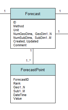
All observations, of all forecasts, are stored in a single forecast point table, which has fixed columns: a forecast ID variable; ‘rank’ which refers to a forecast scenario, such as baseline, or high growth; and a datetime stamp. The remaining columns are 'flexible', in the sense that they refer to different dimensions depending on the forecast. They are: the geographical dimensions (for airports, countries, cities); the sub-dimensions (for age group, aircraft type, international or domestic etc); and, finally, the value. So there are multiple attributes which serve as a key, and a single value. We put in 3 geographical columns and 2 sub-dimension columns at the design stage, and it’s been enough. Some forecasts use all 5, some just a single dimension.

So it’s 'schemaless' in the sense that it has flexible columns. The data types are fixed, dimensions always integer, value being real, but the column name doesn’t tell you what is really stored in there, and the value can be a flight count in one row and a percentage growth, distance, time or something else in the next. Here I'm using 'flexible', because the usage doesn't seem to match up exactly with Martin's use of either 'custom' or 'non-uniform'; maybe closer to non-uniform. 

To manage this welcoming mess of data, we also have what Martin refers to as an ‘attribute table’ (slide 8), which for us is the ‘forecast’ table. It determines what the columns mean in a particular case, and how many are used of the 3 and 2 that are available. The partial schema ;-) below shows these relationships. The attribute table also gives the units that apply to the value column (flights, index (year x = 100), percentage, etc), and most importantly the ‘method’ which determines what type of forecast this ID refers to in the forecast point table (examples in the bulleted list above). 


 (extract)

To give a specific example, the 20-year forecast involves 30 intermediate or output forecasts, as shown below. We keep the inputs separately; there's another 38 of those. The forecasts shown vary from 300 rows to 40 million; from one geo dimension used up to all 5. In fact, we cheat, and 634 is not a geographic dimension even if it's in the geo3 column. The joy of schemaless here is, if it fits, it works.


How?

The main condition, necessary for this to work, is that the key attributes in the forecast point table - rank, geoN, subM, datetime - are each of the same type, regardless of the forecast method, or of what they really represent.

Even to achieve this for something like ‘country’, say, requires some discipline: the raw data have half a dozen different codes and spellings for each country: is that Bosnia-Herzegovina, BOSNIA-HERZEGOVINA, Bosnia-Hercegovina, Bosnia & Herzegovina, BiH, BA or LQ? And they’ve changed over the years, as data suppliers change their minds. We learned the hard way, from a previous implementation that trying to use a 'meaningful' text name is a nightmare, and switched to use a 'business key', an integer not a text name, shortly before we went schemaless.

This goes beyond a ‘factor’ as R would have it, where strings are captured as integers and the values as ‘levels'. It is helped by SAS’s support for user-defined formats. So we have a format ‘FIDTZs', if you want to show or view the integer as a short name, without changing the data, ‘FIDTZl’ for a longer version. (These formats apply to the country, or 'traffic zone' TZ, dimension. Others are defined for other dimensions.)

In addition, we invested in developing the API and the input processes. Every write to, or read from, the forecast table and forecast point table goes through the API. You can even think of each step in the forecast process as ETL ‘extract, transform, load’; each forecast step 'unpacks' one or more (input) 'forecasts' from the forecast point table, using the API, does whatever forecasting is needed at this stage, then packs it back, using the API. But the investment was worth it: we've got a lot of use out of that API over 10 years, and it has needed relatively little maintenance. The modification history has only recently reached 100 items including:  some tweaking to improve speed by passing more work to the server from the desktop; and most recently a switch to implement a test and live version of the tables; otherwise mods largely just adding more known dimensions as the code expanded into new forecast areas. Martin says you need a data access layer, and that's certainly worked for us.

And any external data has to get translated from foreign codes into business key as it is loaded. Again, we have a standard approach, working with input data in MS Excel (which is both flexible and allows that mix of numbers and text which means you can document as you go along), then a fixed import process which understands each input type. It's quite a natural way to work, though maybe more prone to copy-paste or fill-down errors than would be ideal.

For code readability, dimensions are always referred to through macro variable names, so &AATAcEisy instead of 634 in the example above, for the aircraft (AC) entry-into-service year (EISY), in the aircraft assignment tool (AAT). Ok, readability of a sort.


Why?

Earlier toolkits used a ‘distributed’ approach, with input, intermediate and final datasets kept in separate tables in a variety of different places in a set of libraries, or folders. This was traditional for SAS at the time, I think. But we learned the hard way that:
  • A folder structure doesn't look after itself. Some legacy codes still generates files, see example below. Which of these is attached to a published forecast, so we need to keep it, which was a working file? Who knows? A particular issue once more than one person is collaborating on the forecast. Happily even for these datasets, the important ones are saved in our schemaless system, now.
  • Once you've got a forecast, and are trying to work out why it says what is says, 'drilling down' is very time consuming, since each forecast step needs specific handling - since there's no guarantee of consistency of column naming from one step to the next, plus you need to find the right table from each one. With our schemaless version, you just filter the forecast point table for the airport-pair say, that you're interested in, and you can see the trace of how the value was derived.
  • Keeping code components independent is hard, since a column name used in a table creates dependencies throughout the code; in schemaless, the column names are all 'vanilla' geo1, geo2 etc, and each component can rename them to something more meaningful if needed.
  • Similarly, temporary (within component) datasets are clearly separated from lasting ones, since you need to add a forecast method for anything that you want to last, and load it into the forecast table. Maybe this comes naturally in other languages, but not in SAS macro.


And writing each forecast step is easier. Each one begins with the same few lines to look up the forecast ID of the forecast method you want, in the forecast bundle ('forecast set') for this 7-year forecast say. Then a call to unpack it from the datawarehouse. At the other end, the same few lines to align the final dataset with the vanilla column names, and pack it back up into the datawarehouse.

So it's all perfect?

That this schemaless system works is down to the API, the infrastructure and the users. The bits that don't work are down to the API, the infrastructure and the users.

Using the API takes time: we're writing small, or very large, datasets out of the analysis system into an Oracle datawarehouse. That's an extra read and an extra write step compared to keeping it local. And often an extra delete step, since the previous version of the forecast with method X is deleted before the new one is written: forecast methods are unique in a bundle, by design. This definitely affects performance. Even network latency has been a drag at times in our infrastructure. We've tried to improve the delete process, but there must be better ways of sharing out the storage and processing involved here than when we set out.

The graph shows timings from the main part of the 7-year forecast. On a test of a single run, out of 15 minutes real time, 55% is spent packing up the results through the API. The two longest processes, C211 and C206, each spend more than 50% of their time packing up into our semi-schemaless store. The high cost is clear.


The data we want to store in future is only likely to get larger, if we add more forecast types to our existing ensemble process, or tackle uncertainty more through hypothetical outcome plots than scenarios. So the performance challenge is going to get more difficult.

As Martin says, custom columns cause sparse tables - you can see how sparse in the table above. But I haven't worked out how to evaluate whether sparseness is really part of our performance problem. If the alternative is a single column with embedded structure, maybe that's getting easier to handle (r package purr::transpose anyone?).

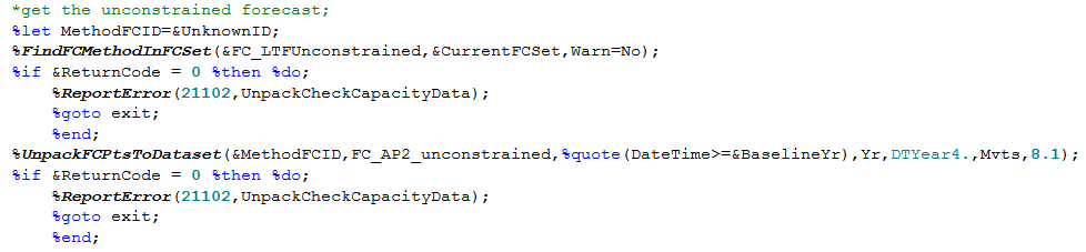
The API invocations are routine, so quick to write, but ugly and long which doesn't do much for readability, or for those times when you're writing scratch code for a quick look at a dataset. See the example below. Why not wrap all this in a single call? Mostly, because of the difficulty of passing the parameters to the %unpack call, since they vary a lot from one instance to the next. In particular the last 4 rename and format the DateTime and Value columns: move from vanilla names to meaningful ones. This would be easier in R, for example. And easier with a bit more metadata: if the system automatically associated the forecast method &FC_LTFUnconstrained with the fact that the right column names are 'Yr', formatted as '2019' etc. Why not do the same for the geo & sub dimension columns at the same time? This would tip the balance from being semi-schemaless to having a sort of 'meta-schema', one layer up from the data structure itself.

You could even exploit the fact that we have a data access layer in place to migrate to a different database structure, where there is one ForecastPoint table for each forecast method. Currently that means moving to 175 different tables, since there are 175 different forecast methods. Doing this at the data end would cut the sparseness problem, but getting the full benefit would involve more code changes (to give the different tables more meaningful column names, for example). 


And that ">=BaselineYr" filter? We're still doing it locally rather than in the datawarehouse.

The first cookbook I remember as a kid had a motto in the front: tidy up as you go along, it's easier in the end. We try to have a culture of clearing up as we go, but we've still accumulated 5,500 forecasts in 800 bundles ('forecast sets'). It may be easier with our schemaless system to tidy up, but someone still has to do it occasionally. Even with best intentions, the kitchen can end up a mess when you're busy and having fun. On the to-do list is improvements to the metadata for better flagging of published forecasts, and better protection than the simple locks we implemented, which haven't stopped some mistakes.

Some of that is down to knowledge transfer. As a user or a coder, it takes a little time to get used to this way of working. And the rare mistakes - usually a mistaken over-write - have usually come down to lack of familiarity, or not taking enough time to explain the system.

Using the business keys also takes effort, and requires regular reinforcement. Not to mention the data management side. Do we need to be more open to other data? That's a big enough topic  for another time.

There were parts of the API that were built, or built as stubs, that we've never used. For example, we have a switch for using a private or a shared set of forecast and forecast point tables. Not used in years - though now we've implemented something similar, to align with the dev-test-live version of the datawarehouse. Other parts of the system, such as the error checking for availability of datasets (example above), add to the length and complexity, but are very rarely triggered, and when they are, the reports are lost in the noise of other logging from the system. Could do better.

Conclusion

Whether we are truly 'schemaless' in the end is beside the point. We adopted a flexible approach with an explicit meta-schema and it has served us well over the last 10 or 12 years. The main issue is performance.

In re-engineering our forecast toolset, it would be hard to start with a completely clean sheet. Our legacy approach to structuring and handling data for the forecasts still feels like a good foundation for building the new system, but that's not to the exclusion of some adaptation to exploit the data tools that are now available. 


(Updated 22 August with timings chart, and with more reliable images.)